複数の学習済みモデルを評価する。評価項目と各コードを紹介。

結論
- 学習済みモデルの評価方法をまとめました。
- 作成したコードと出力結果を紹介します。
はじめに
深層学習で得られたモデル群の評価について、
- どのような評価軸があるのか
- 実際にどのようなコードを書けばよいのか
をまとめました。
例えば学習中であればepoch毎の損失値や精度を確認することができますが、学習が終わってしまえばどのようにそれら複数モデルの性能を評価すればよいのか、ということが気になると思います。
どのモデルが最も良いモデルなのかを判断するためには、評価方法を知っておく必要があります。
評価の種類
学習済みのモデルを評価する評価項目
AUC-ROC (Area Under the Curve – Receiver Operating Characteristic)
モデルの性能を示すグラフで、偽陽性率に対する真陽性率をプロットしたものです。
AUC(曲線下面積)が1に近いほどモデルの性能が良いとされます。AUCを省略する場合もあります。
精度(Accuracy)
モデルが正確に予測できた割合を示します。
1に近いほどモデルの性能が良いとされます。
F1スコア (F1 Score)
汎化性能のバランスの良さを示す指標です。
1に近いほどモデルの性能が良いとされます。
モデルの解釈可能性 (Model Interpretability)
モデルがどのように予測を行っているのかを理解するための指標や手法です。
SHAP、GradCAMなどがあり、視覚的に確認することが出来ます。
他に テスト損失 (汎化損失) があります。
混同行列(Confusion Matrix)
混同行列はモデルの予測結果を正解と不正解、正例と負例に分けて表示したもので、分類問題の結果を詳細に表示するための「表」です。
| 予測: Positive | 予測: Negative | |
|---|---|---|
| 実際: Positive | True Positive | False Negative |
| 実際: Negative | False Positive | True Negative |
行は実際のクラスを、列は予測されたクラスを示します。
この行列は以下の4つの部分から成り立っています。
- True Positive (TP): 正のクラスを正しく正と予測した数
- True Negative (TN): 負のクラスを正しく負と予測した数
- False Positive (FP): 負のクラスを誤って正と予測した数(偽陽性)
- False Negative (FN): 正のクラスを誤って負と予測した数(偽陰性)
混同行列から適合率と再現率を求め、その結果を使ってF1スコアを求めることができます。
適合率(Precision)
正と予測されたサンプルのうち、実際に正であったサンプルの割合を示します。
「予測がどれだけ信頼できるか」を示し、以下の式で計算されます。
$$
\text{{Precision}} = \frac{{\text{{TP}}}}{{\text{{TP}} + \text{{FP}}}}
$$
再現率(Recall)
実際の正のサンプルのうち、正と予測されたサンプルの割合を示します。
「正のサンプルをどれだけ捉えられるか」を示し、以下の式で計算されます。
$$
\text{{Recall}} = \frac{{\text{{TP}}}}{{\text{{TP}} + \text{{FN}}}}
$$
F1スコア
適合率と再現率の調和平均であり、これら2つの指標のバランスを示します。
$$
\text{{F1 Score}} = \frac{{2 \times (\text{{Precision}} \times \text{{Recall}})}}{{\text{{Precision}} + \text{{Recall}}}}
$$
F1スコアなどの指標が重要な理由
クラスの不均衡が存在する場合、単純な精度(Accuracy)だけではモデルの性能を正確に評価できません。
例えば99%のサンプルがクラスA、1%のサンプルがクラスBの場合、すべてのサンプルをクラスAと予測するだけで精度は99%になります。しかしこれはクラスBのサンプルを全く予測できていないという問題をはらんでいるかもしれません。
このような場合、適合率・再現率・F1スコアなどの指標を使用することで、モデルの性能をより正確に評価することができます。
実例
評価用データセット
学習に用いたデータセットとは異なる約5000枚の顔画像を含むデータセットを用意しました。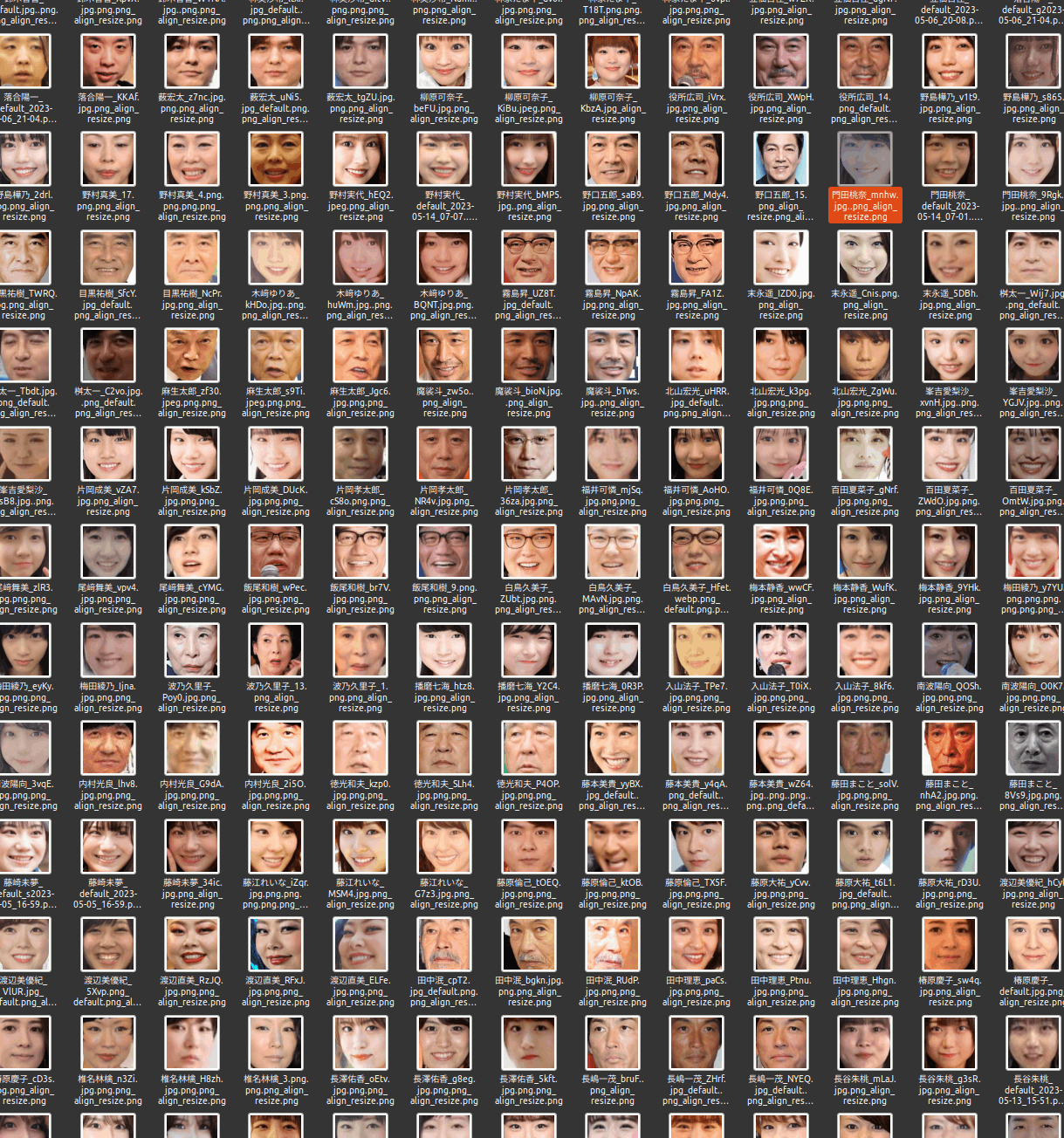
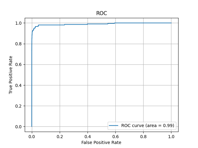
ROC曲線
"""make_ROC_graph.py"""
import os
from itertools import combinations
import sys
import numpy as np
import onnx
import onnxruntime as ort
import torchvision.transforms as transforms
from PIL import Image
from sklearn.metrics import roc_curve, auc
import matplotlib.pyplot as plt
import cupy as cp


sys.path.append('/home/terms/bin/FACE01_IOT_dev')
from face01lib.utils import Utils  # type: ignore
Utils_obj = Utils()

model_name = 'efficientnetv2_arcface.onnx'

# 画像の前処理を定義
mean_value = [0.485, 0.456, 0.406]
std_value = [0.229, 0.224, 0.225]
transform = transforms.Compose([
    transforms.Resize((224, 224)),
    transforms.ToTensor(),
    transforms.Normalize(
        mean=mean_value,
        std=std_value
    )
])

# ONNXモデルをロード
onnx_model = onnx.load(model_name)
ort_session = ort.InferenceSession(model_name)

# 署名表示
for prop in onnx_model.metadata_props:
    if prop.key == "signature":
        print(prop.value)

# 入力名を取得
input_name = onnx_model.graph.input[0].name

# 推論対象の画像ファイルを取得
image_dir = "predict_test"
image_files = [os.path.join(image_dir, f) for f in os.listdir(image_dir) if f.endswith('.png')]

# 類似度判断の関数
def is_same_person(embedding1, embedding2):
    embedding1 = cp.asarray(embedding1).flatten()
    embedding2 = cp.asarray(embedding2).flatten()
    cos_sim = cp.dot(embedding1, embedding2) / (cp.linalg.norm(embedding1) * cp.linalg.norm(embedding2))
    return cos_sim.get()  # .get()を追加


# 画像を読み込み、前処理を行い、モデルで推論を行う
embeddings_dict = []
i = 0
for image_file in image_files:
    i += 1
    # 50回に1回、CPU温度を取得
    if i % 50 == 0:
        # CPU温度が72度を超えていたら待機
        Utils_obj.temp_sleep()
        i = 0
    name = os.path.splitext(os.path.basename(image_file))[0]
    # nameを'_'で分割して、ラベルを取得
    name = name.split('_')[0]
    image = Image.open(image_file).convert('RGB')
    image = transform(image)
    image = image.unsqueeze(0)  # バッチ次元を追加
    image = image.numpy()
    embedding = ort_session.run(None, {input_name: image})[0]  # 'input'をinput_nameに変更
    # name: embeddingの辞書を作成
    dict = {name: embedding}
    embeddings_dict.append(dict)

# embeddings_dictの各要素のペアを作成
pair = list(combinations(embeddings_dict, 2))
# pairのkeyが同一ならlabelを1、異なれば0とする
labels = [1 if list(pair[i][0].keys())[0] == list(pair[i][1].keys())[0] else 0 for i in range(len(pair))]
# pairの各要素の類似度を計算
scores = [is_same_person(pair[i][0][list(pair[i][0].keys())[0]], pair[i][1][list(pair[i][1].keys())[0]]) for i in range(len(pair))]
# labelsとscoresを結合
labels_scores = list(zip(labels, scores))

# labels_scoresをもとにROC曲線の計算
fpr, tpr, thresholds = roc_curve(labels, scores)

# AUCの計算
roc_auc = auc(fpr, tpr)

# ROC曲線の描画
plt.plot(fpr, tpr, label='ROC curve (area = %.2f)'%roc_auc)
plt.xlabel('False Positive Rate')
plt.ylabel('True Positive Rate')
plt.title('ROC')
plt.grid(True)
plt.legend(loc="lower right")  # 凡例の表示
plt.show()
input("Enterで処理を終了します")
精度と閾値の関係
from itertools import combinations
import os
import sys
import numpy as np
import onnx
import onnxruntime as ort
import torchvision.transforms as transforms
from PIL import Image
from sklearn.metrics import accuracy_score
import matplotlib.pyplot as plt
import cupy as cp


sys.path.append('/home/terms/bin/FACE01_IOT_dev')
from face01lib.utils import Utils  # type: ignore
Utils_obj = Utils()

model_name = 'efficientnetv2_arcface.onnx'

# 画像の前処理を定義
mean_value = [0.485, 0.456, 0.406]
std_value = [0.229, 0.224, 0.225]
transform = transforms.Compose([
    transforms.Resize((224, 224)),
    transforms.ToTensor(),
    transforms.Normalize(
        mean=mean_value,
        std=std_value
    )
])

# ONNXモデルをロード
onnx_model = onnx.load(model_name)
ort_session = ort.InferenceSession(model_name)

# 署名表示
for prop in onnx_model.metadata_props:
    if prop.key == "signature":
        print(prop.value)

# 入力名を取得
input_name = onnx_model.graph.input[0].name

# 推論対象の画像ファイルを取得
image_dir = "predict_test"
image_files = [os.path.join(image_dir, f) for f in os.listdir(image_dir) if f.endswith('.png')]

# 類似度判断の関数
def is_same_person(embedding1, embedding2):
    embedding1 = cp.asarray(embedding1).flatten()
    embedding2 = cp.asarray(embedding2).flatten()
    cos_sim = cp.dot(embedding1, embedding2) / (cp.linalg.norm(embedding1) * cp.linalg.norm(embedding2))
    return cos_sim

# 画像を読み込み、前処理を行い、モデルで推論を行う
embeddings_dict = []
i = 0
for image_file in image_files:
    i += 1
    # 50回に1回、CPU温度を取得
    if i % 50 == 0:
        # CPU温度が72度を超えていたら待機
        Utils_obj.temp_sleep()
        i = 0
    name = os.path.splitext(os.path.basename(image_file))[0]
    # nameを'_'で分割して、ラベルを取得
    name = name.split('_')[0]
    image = Image.open(image_file).convert('RGB')
    image = transform(image)
    image = image.unsqueeze(0)  # バッチ次元を追加
    image = image.numpy()
    embedding = ort_session.run(None, {input_name: image})[0]  # 'input'をinput_nameに変更
    # name: embeddingの辞書を作成
    dict = {name: embedding}
    embeddings_dict.append(dict)

# embeddings_dictの各要素のペアを作成
pair = list(combinations(embeddings_dict, 2))
# pairのkeyが同一ならlabelを1、異なれば0とする
labels = [1 if list(pair[i][0].keys())[0] == list(pair[i][1].keys())[0] else 0 for i in range(len(pair))]
# pairの各要素の類似度を計算
scores = [is_same_person(pair[i][0][list(pair[i][0].keys())[0]], pair[i][1][list(pair[i][1].keys())[0]]) for i in range(len(pair))]
# labelsとscoresを結合
labels_scores = list(zip(labels, scores))

# 閾値の範囲を設定
thresholds = np.arange(-1, 1, 0.01)

# 各閾値でのAccuracyを計算
accuracies = []
predictions = []
# 閾値を変えながら、labels_scoresの各要素を正解ラベルと予測ラベルに分ける
for threshold in thresholds:
    for label, score in labels_scores:
        if score >= threshold:
            predictions.append(1)
        else:
            predictions.append(0)
    accuracy = accuracy_score(labels, predictions)
    accuracies.append(accuracy)
    predictions.clear()

# グラフを作成
plt.plot(thresholds, accuracies)
plt.xlabel('Threshold')
plt.ylabel('Accuracy')
plt.title('Accuracy vs. Threshold')
plt.grid(True)
plt.show()
input("Enterで処理を終了します")
閾値の選択基準(精度とF1スコア)
import os
from itertools import combinations
import sys
import numpy as np
import onnx
import onnxruntime as ort
import torchvision.transforms as transforms
from PIL import Image
from sklearn.metrics import accuracy_score, confusion_matrix, precision_score, recall_score, f1_score
import cupy as cp


sys.path.append('/home/terms/bin/FACE01_IOT_dev')
from face01lib.utils import Utils  # type: ignore
Utils_obj = Utils()

model_name = 'efficientnetv2_arcface.onnx'

# 画像の前処理を定義
mean_value = [0.485, 0.456, 0.406]
std_value = [0.229, 0.224, 0.225]
transform = transforms.Compose([
    transforms.Resize((224, 224)),
    transforms.ToTensor(),
    transforms.Normalize(
        mean=mean_value,
        std=std_value
    )
])

# ONNXモデルをロード
onnx_model = onnx.load(model_name)
ort_session = ort.InferenceSession(model_name)

# 署名表示
for prop in onnx_model.metadata_props:
    if prop.key == "signature":
        print(prop.value)

# 入力名を取得
input_name = onnx_model.graph.input[0].name

# 推論対象の画像ファイルを取得
image_dir = "predict_test"
image_files = [os.path.join(image_dir, f) for f in os.listdir(image_dir) if f.endswith('.png')]

# 類似度判断の関数
def is_same_person(embedding1, embedding2):
    embedding1 = cp.asarray(embedding1).flatten()
    embedding2 = cp.asarray(embedding2).flatten()
    cos_sim = cp.dot(embedding1, embedding2) / (cp.linalg.norm(embedding1) * cp.linalg.norm(embedding2))
    return cos_sim


# 画像を読み込み、前処理を行い、モデルで推論を行う
embeddings_dict = []
i = 0
for image_file in image_files:
    i += 1
    # 50回に1回、CPU温度を取得
    if i % 50 == 0:
        # CPU温度が72度を超えていたら待機
        Utils_obj.temp_sleep()
        i = 0
    name = os.path.splitext(os.path.basename(image_file))[0]
    # nameを'_'で分割して、ラベルを取得
    name = name.split('_')[0]
    image = Image.open(image_file).convert('RGB')
    image = transform(image)
    image = image.unsqueeze(0)  # バッチ次元を追加
    image = image.numpy()
    embedding = ort_session.run(None, {input_name: image})[0]  # 'input'をinput_nameに変更
    # name: embeddingの辞書を作成
    dict = {name: embedding}
    embeddings_dict.append(dict)

# embeddings_dictの各要素のペアを作成
pair = list(combinations(embeddings_dict, 2))
# pairのkeyが同一ならlabelを1、異なれば0とする
labels = [1 if list(pair[i][0].keys())[0] == list(pair[i][1].keys())[0] else 0 for i in range(len(pair))]
# pairの各要素の類似度を計算
scores = [is_same_person(pair[i][0][list(pair[i][0].keys())[0]], pair[i][1][list(pair[i][1].keys())[0]]) for i in range(len(pair))]
# labelsとscoresを結合
labels_scores = list(zip(labels, scores))

# Calculate accuracy, confusion matrix, precision, recall, and F1 score for different thresholds
thresholds = np.arange(0.1, 1.1, 0.1)  # 0.1から1.0まで0.1刻みで閾値を設定
true_labels = [label for label, _ in labels_scores]

for threshold in thresholds:
    predicted_labels = [1 if score > threshold else 0 for _, score in labels_scores]

    accuracy = accuracy_score(true_labels, predicted_labels)
    print(f'Accuracy for threshold {threshold}:', accuracy)

    # Calculate confusion matrix
    cm = confusion_matrix(true_labels, predicted_labels)
    print(f'Confusion Matrix for threshold {threshold}:\n', cm)

    # Calculate precision
    precision = precision_score(true_labels, predicted_labels)
    print(f'Precision for threshold {threshold}:', precision)

    # Calculate recall
    recall = recall_score(true_labels, predicted_labels)
    print(f'Recall for threshold {threshold}:', recall)

    # Calculate F1 score
    f1 = f1_score(true_labels, predicted_labels)
    print(f'F1 Score for threshold {threshold}:', f1)

    print('--------------------------')
Accuracy for threshold 0.1: 0.9109571989403467
Confusion Matrix for threshold 0.1:
[[427917 41843]
[ 4 201]]
Precision for threshold 0.1: 0.004780705927123965
Recall for threshold 0.1: 0.9804878048780488
F1 Score for threshold 0.1: 0.009515018106937442
--------------------------
Accuracy for threshold 0.2: 0.9927781856095667
Confusion Matrix for threshold 0.2:
[[466382 3378]
[ 16 189]]
Precision for threshold 0.2: 0.05298570227081581
Recall for threshold 0.2: 0.9219512195121952
F1 Score for threshold 0.2: 0.10021208907741251
--------------------------
Accuracy for threshold 0.30000000000000004: 0.998982902982137
Confusion Matrix for threshold 0.30000000000000004:
[[469317 443]
[ 35 170]]
Precision for threshold 0.30000000000000004: 0.27732463295269166
Recall for threshold 0.30000000000000004: 0.8292682926829268
F1 Score for threshold 0.30000000000000004: 0.41564792176039117
--------------------------
Accuracy for threshold 0.4: 0.9997318949283457
Confusion Matrix for threshold 0.4:
[[469700 60]
[ 66 139]]
Precision for threshold 0.4: 0.6984924623115578
Recall for threshold 0.4: 0.6780487804878049
F1 Score for threshold 0.4: 0.6881188118811881
--------------------------
Accuracy for threshold 0.5: 0.9997531731086358
Confusion Matrix for threshold 0.5:
[[469748 12]
[ 104 101]]
Precision for threshold 0.5: 0.8938053097345132
Recall for threshold 0.5: 0.4926829268292683
F1 Score for threshold 0.5: 0.6352201257861636
--------------------------
Accuracy for threshold 0.6: 0.9996616769333887
Confusion Matrix for threshold 0.6:
[[469759 1]
[ 158 47]]
Precision for threshold 0.6: 0.9791666666666666
Recall for threshold 0.6: 0.22926829268292684
F1 Score for threshold 0.6: 0.37154150197628455
--------------------------
Accuracy for threshold 0.7000000000000001: 0.9996191205728087
Confusion Matrix for threshold 0.7000000000000001:
[[469760 0]
[ 179 26]]
Precision for threshold 0.7000000000000001: 1.0
Recall for threshold 0.7000000000000001: 0.12682926829268293
F1 Score for threshold 0.7000000000000001: 0.2251082251082251
--------------------------
Accuracy for threshold 0.8: 0.9995808198482866
Confusion Matrix for threshold 0.8:
[[469760 0]
[ 197 8]]
Precision for threshold 0.8: 1.0
Recall for threshold 0.8: 0.03902439024390244
F1 Score for threshold 0.8: 0.07511737089201878
--------------------------
Accuracy for threshold 0.9: 0.9995659251220835
Confusion Matrix for threshold 0.9:
[[469760 0]
[ 204 1]]
Precision for threshold 0.9: 1.0
Recall for threshold 0.9: 0.004878048780487805
F1 Score for threshold 0.9: 0.009708737864077669
--------------------------
Accuracy for threshold 1.0: 0.9995637973040545
Confusion Matrix for threshold 1.0:
[[469760 0]
[ 205 0]]Grad-CAMによる可視化
import numpy as np
import torch
from PIL import Image
from torchvision import transforms
import matplotlib.pyplot as plt
import cv2
import timm
from torch import nn
from pytorch_grad_cam import GradCAM

# モデルの定義
class CustomModel(nn.Module):
    def __init__(self, embedding_dim=512):
        super(CustomModel, self).__init__()

        # EfficientNet V2の事前学習済みモデルを取得し、trunkとして定義
        self.trunk = timm.create_model('tf_efficientnetv2_b0', pretrained=True)
        num_features = self.trunk.classifier.in_features

        # trunkの最終層にembedding_size次元のembedder層を追加
        self.trunk.classifier = nn.Linear(num_features, embedding_dim)

    def forward(self, x):
        return self.trunk(x)

input_image = "shap.png"

# 画像の前処理を定義
mean_value = [0.485, 0.456, 0.406]
std_value = [0.229, 0.224, 0.225]
transform = transforms.Compose([
    transforms.Resize((224, 224)),
    transforms.ToTensor(),
    transforms.Normalize(
        mean=mean_value,
        std=std_value
    )
])

# モデルのインスタンスを作成
pytorch_model = CustomModel()

# モデルの状態辞書をロード
state_dict = torch.load("best_model_169epoch_512diml.pth")

# 状態辞書をモデルに適用
pytorch_model.load_state_dict(state_dict)

# モデルを評価モードに設定
pytorch_model.eval()

# Grad-CAMのための準備
target_layer = pytorch_model.trunk.blocks[-1]

# Grad-CAMのインスタンスを作成
cam = GradCAM(pytorch_model, target_layer, use_cuda=False)

# 画像の読み込みと前処理
image = Image.open(input_image)
input_tensor = transform(image) # 前処理の適用
input_tensor = input_tensor.unsqueeze(0) # バッチ次元の追加

# Grad-CAMの実行
target_category = None
grayscale_cam = cam(input_tensor, target_category)

# ヒートマップの作成
grayscale_cam = grayscale_cam[0, :]
heatmap = cv2.applyColorMap(np.uint8(grayscale_cam * 255), cv2.COLORMAP_JET)
heatmap = cv2.cvtColor(heatmap, cv2.COLOR_BGR2RGB)  # 追加:ヒートマップの色の順序をRGBに変更

# 画像の読み込み
original_image = cv2.imread(input_image, cv2.IMREAD_COLOR)
original_image = cv2.cvtColor(original_image, cv2.COLOR_BGR2RGB)

# 画像とヒートマップのサイズが同じであることを確認
assert original_image.shape == heatmap.shape

# 画像とヒートマップをアルファブレンド
alpha = 0.5
blended = cv2.addWeighted(original_image, alpha, heatmap, 1 - alpha, 0)

# 結果を表示
plt.imshow(blended)
plt.show()
モデルの評価
以上の結果から、モデルの評価を行います。
ROC曲線
グラフから、訓練とテストの精度とF1スコアがともに高いレベルに達していることが視覚的に確認できます。
汎化性能が高く、未見のデータに対しても良好な予測性能を持つことを示しています。
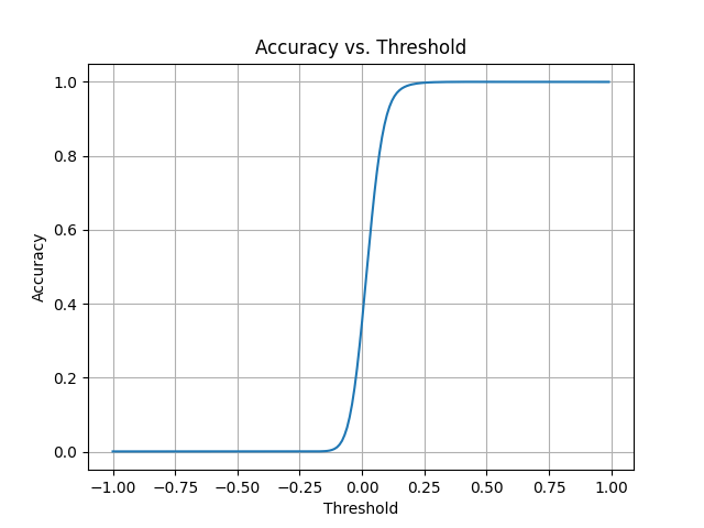
精度とF1スコア
グラフから、訓練とテストの精度とF1スコアがともに高いレベルに達していることが視覚的に確認できます。
汎化性能が高く、未見のデータに対しても良好な予測性能を持つことを示しています。

閾値の選択
最適な閾値をグラフから読み取ることが出来ます。訓練データに対する精度とF1スコアのグラフから、閾値を0.5に設定すると、モデルの性能が最も高くなることが分かります。
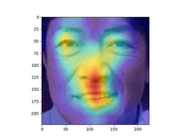
Grad-CAM
Grad-CAMの結果からは、モデルがどのようなな特徴を「見て」分類に利用していることが分かります。
結果から見ると、目の位置、鼻筋から口にかけて注目しているようです。この結果は精度の高さを裏付けます。
以上の情報に基づき、計測した学習モデルはおおむね「良好」と評価できます。
ROC曲線と精度・F1スコアのグラフから、モデルがデータをうまく学習し、予測に成功していることが示唆されます。
次に、閾値の選択によりモデルの性能を最適化できることが視覚的に確認できます。
最後に、Grad-CAMにより、モデルが重要な特徴を学習していることがわかります。
これらの要素からこの学習モデルは「全体的に良好」と評価することが出来ます。
複数モデルを評価する場合、これらの結果から「F1スコアがより1に近いモデル」を選択することが最良と思われます。
See also
https://github.com/yKesamaru/FACE01_SAMPLE
- Face recognition library that integrates various functions and can be called from Python.
AUC-ROC
https://qiita.com/TsutomuNakamura/items/ef963381e5d2768791d4
混同行列
https://qiita.com/TsutomuNakamura/items/a1a6a02cb9bb0dcbb37f
CAM
https://arxiv.org/pdf/1610.02391.pdf
https://zenn.dev/iq108uni/articles/7269a1b72f42be
https://tech-blog.abeja.asia/entry/cam-202203